Today we will see possible ways to estimate which parts of a city are relatively better or worse off than average by using the census variables we gathered in our previous post along with available income open data on a city basis.

First of all, let's download the tax open data from here: http://www1.finanze.gov.it/finanze3/analisi_stat/index.php?opendata=yes
What we are looking for is "2017 a.i. 2016 / IRPEF / Persone fisiche / Tutte le tipologie di contribuenti", which will give us tax data on a city basis.
Let's load the file in Alteryx and select the columns we need, in this case we'll just take the following variables:

- Codice ISTAT Comune is the city code, which we'll need to link with the Census varibles.
- Denominazione Comune is the City name
- Sigla Provincia is the city's Province
- Regione is the City's Region
- Reddito imponibile - Frequenza is the amount of tax payers actually paying income
- Reddito imponibile - Ammontare in euro is the total amount of taxable income
Note that this is not what people is actually earning but only the taxable part. While not a perfect representation of income, this is still useful enough as people below the taxable threshold are mostly not earning enough for any meaningful living, which means they are usually dependent on someone else.
As a first cautionary note, this exercise is not meant to be an accurate representation of income for every area, just a relative estimate of what variables could indicate a certain area having a higher or lower income than average so if you happen to live in one of the analized areas don't assume to be able to use the resulting number to know how much people around you are actually earning!
Another cautionary note is that we're looking at income from 2016, while the census data is from 2011, meaning that there will be cities without census data, which will be ignored for this article's purpose.
We'll now simply estimate average income by dividing the total taxable income by the number of tax payers. Let's also sort it and see which cities are better off in average:

Some might have been expecting higher numbers or other cities on top, but remember this is just taxable income (missing at least 8000€ per person as income below that amount is not taxed, plus other exemptions I suppose) and not total income or wealth.
How do we link this data with the Census in a meaningful way?
We'll try two ways, the first one is checking deviation from average, while the second one will be using machine learning to estimate.
First of all, let's take our census data and average it by city:

Now that we have the averaged census values by city, we can do a simple correlation analysis between those and the average income via the Pearson correlation tool, from which we will take the 20 strongest variables, sorted by absolute value:

Looks like we have some decent correlations, although of course not all are useable as some are extremely correlated to each other (for example, maschi analfabeti is the number or illiterate males, which is a subdivision of analfabeti or illiterate people in general). Still, we have enough to pick some interesting variables.
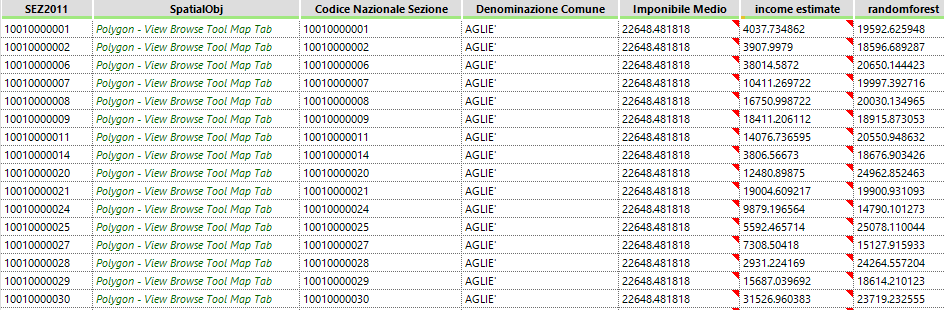
Next, we will join the census areas with the average values and calculate the ratios for some variables:

To calculate the income estimate we'll multiply the value by (1+ratio) where the correlation is positive and divide for the ones where it's negative.
Let's try with what happens with a few variables:

This is a first example of estimate, might be a little pessimistic as we put more negative correlation than positive but at least one district is quite a bit above average, so it might be possible that income is actually highly concentrated.
As you can see, the distribution is quite irregular and the extreme variations are likely because of the low number of variables and the very rough chosen method (which is better for far simpler distributions).
How would a more robust algorithm fare?
Let's try a Random Forest:
As setting, we'll use 500 trees, 90% of the records available for each tree and a minimum leaf size of 100 to lessen overfitting risk, using all census variables:
Definitely less extreme as variation, although how realistic is to be seen.
The accuracy of both estimates is also limited by the fact that we are using only the raw data, which while meaningful rarely explains the full story by itself.
This concludes our article, stay tuned for the next part about using feature engineering and visualization!
No comments:
Post a Comment